In this post we’ll look at some cool algorithms, methods & formulas that solve interesting problems.

Fibonacci Sphere
- Example
- Code
Sphere Projection
Project UV Map onto Sphere
Smooth Minimum
Random Number with Bias

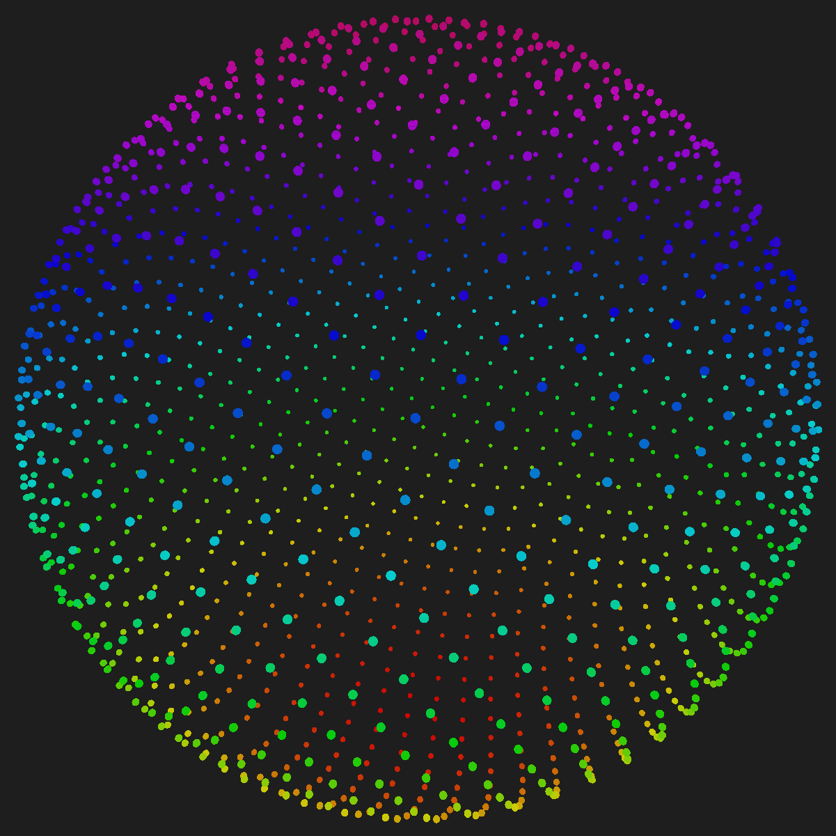
Fibonacci Sphere

This algorithm allows us to generate a sphere made of N points that are pretty evenly distributed. I first learned about this algorithm here, which is also where the code comes from.

Fibonacci Sphere Example

Fibonacci Sphere Code

  
let radius = 300;
let numOfPoints = 1500;

let goldenRatio = (1 + Math.sqrt(5)) / 2;
let angleIncrement = 2*Math.PI * goldenRatio;

for (let i = 0; i < numOfPoints; ++i) {
	let t = i / numOfPoints;
	let angle1 = Math.acos(1 - 2*t);
	let angle2 = angleIncrement * i;

	let x = Math.sin(angle1) * Math.cos(angle2);
	let y = Math.sin(angle1) * Math.sin(angle2);
	let z = Math.cos(angle1);
}

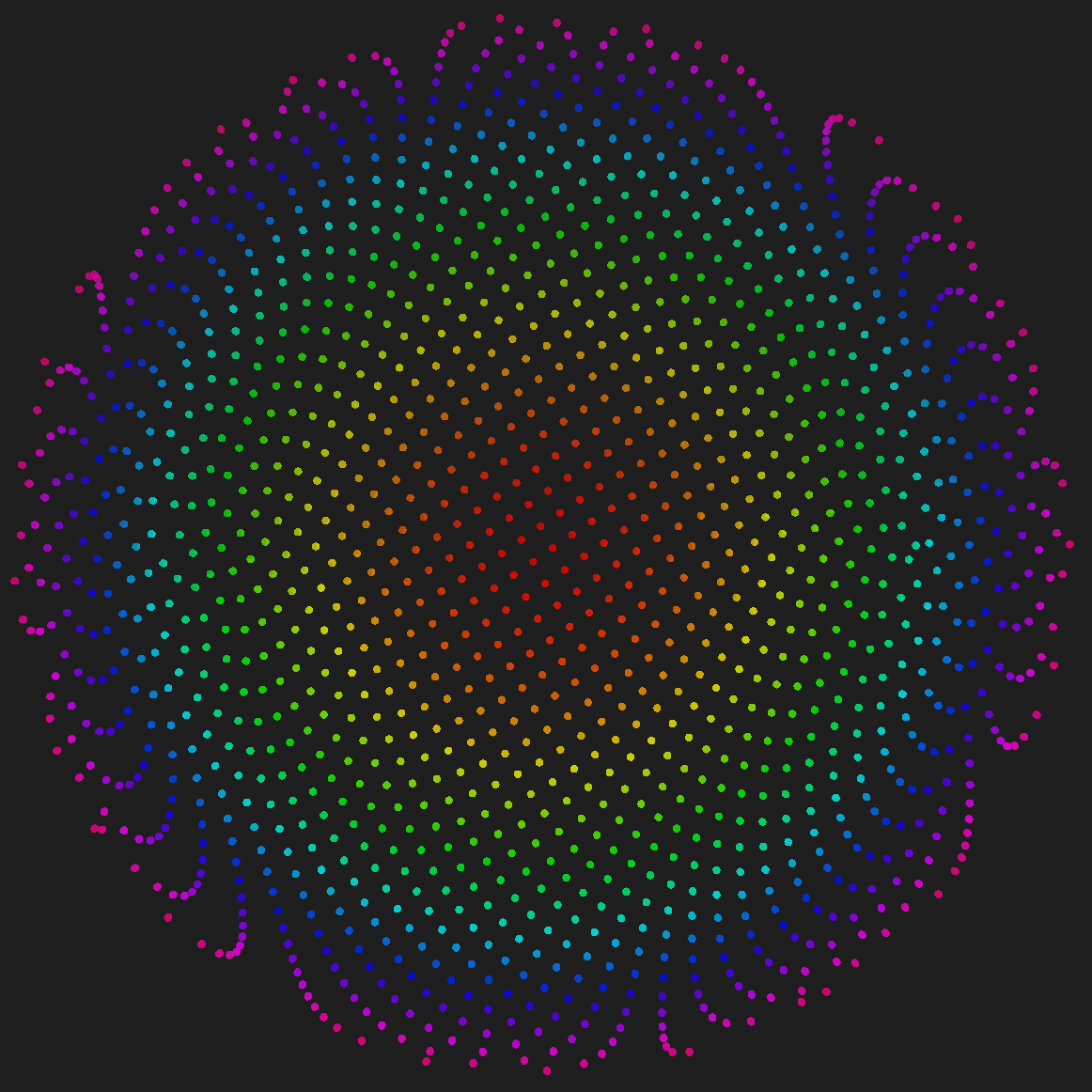
Sphere Projection

This section will look at projecting points from a sphere onto a 2d plane using three different methods. The examples below will use the $X$, $Y$, $Z$ points generated by the Fibonacci Sphere code above.

The following sphere was used in the below examples:

UV Mapping

The variables $U$ and $V$ are used to represent the $X$ and $Y$ values in 2d so that they don’t get confused with the $X$, $Y$, $Z$ values of the 3d coordinate used as input.

The inputs values $\left\{ X,Y,Z \in \left[-1, 1\right] \subset \mathbb{R}\right\}$, and the output values $\left\{ U,V \in \left[0, 1\right] \subset \mathbb{R} \right\}$.

$U = 0.5 + \arctan2(X, Z) / 2\pi$

$V = 0.5 - \arcsin(Y) / \pi$

The formula can be adjusted to the following so that $\left\{ U,V \in \left[-1, 1\right] \subset \mathbb{R} \right\}$:

$U = 2\arctan2(X, Z) / 2\pi$

$V = 2\arcsin(Y) / \pi$

Polar Coordinates Method 1

Instead of projecting the sphere on a square, we can project it onto a circle instead.

$r = \sqrt{X^2 + (Y+1)^2 + Z^2}$

$U = r\cos(\arctan2(X, Z))$

$V = r\sin(\arctan2(X, Z))$

The above formula is obtained by combing the Spherical¹ and Polar² coordinate system formulas. Here is how it’s done.

We can convert from the Polar coordinates to Cartesian coordinates using the following:

$U = r\cos(\varphi)$

$V = r\sin(\varphi)$

To get $\varphi$ we use the Spherical coordinate formula. Since we want $\varphi$ to be $\left[0,2\pi\right]$, we want to use the azimuthal angle, which can be calculated using:

$\varphi = \arctan2(X, Z)$

$X$ and $Z$ are used in the above line because the y-axis is vertical our 3d space.

Finally we need to calculate the radius $r$, which can be done by using the Spherical coordinate radius formula. The only adjustment is that we need to calculate the distance from the bottom of the sphere $(0,-1,0)$, otherwise we will end up with all the points mapped onto the perimeter of circle, rather than inside it.

$r = \sqrt{X^2 + (Y+1)^2 + Z^2}$

Polar Coordinates Method 2

We can do a slight modification to the above formula for calculating the radius, by just using the $Y$ value. Since $\left\{ Y \in \left[-1, 1\right] \subset \mathbb{R} \right\}$, and radii can’t be negative, we need to map $Y$ so $\left\{ Y \in \left[0, 1\right] \subset \mathbb{R} \right\}$. This is what $Y_{m}$ does below:

$Y_{m} = (Y+1) / 2$

$U = Y_{m}\cos(\arctan2(X, Z))$

$V = Y_{m}\sin(\arctan2(X, Z))$

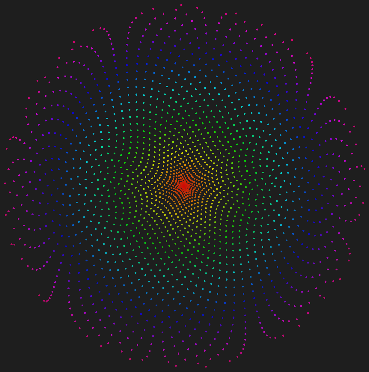
While the above formula is nice, there is an obvious clustering of points at the center of the circle. We can fix this by making the radius equal $\sqrt{Y_{m}}$ instead of just $Y_{m}$. An explanation of why this works can be here. The range of $U$ and $V$ stay the same, as $Y_{m}$ has the range $\left[0, 1\right]$ and $\sqrt{Y_{m}}$ also has the range $\left[0, 1\right]$, since $\sqrt{0} = 0$ and $\sqrt{1} = 1$.

$Y_{m} = \sqrt{(y+1) / 2}$

$U = Y_{m}\cos(\arctan2(X, Z))$

$V = Y_{m}\sin(\arctan2(X, Z))$

Even with this adjustment, the output will still be slightly different from the previous method, as the $X$ and $Z$ values were not taken into account when calculating the radius.

Project UV Map onto Sphere

This is the reverse transformation to the UV Mapping we did above. For the below equations, the input values $\left\{ U,V \in \left[0, 1\right] \subset \mathbb{R} \right\}$, and the output values $\left\{ X,Y,Z \in \left[-1, 1\right] \subset \mathbb{R}\right\}$.

$r = \cos(\pi(0.5-V))$

$X = r\sin(2\pi(U-0.5))$

$Y = \sin(\pi(0.5-V))$

$Z = r\cos(2\pi(U-0.5))$

Smooth Minimum

The smooth min function as the name implies allows us to take the minimum of two values smoothly, which works to remove sharp edges when blending functions and shapes³.

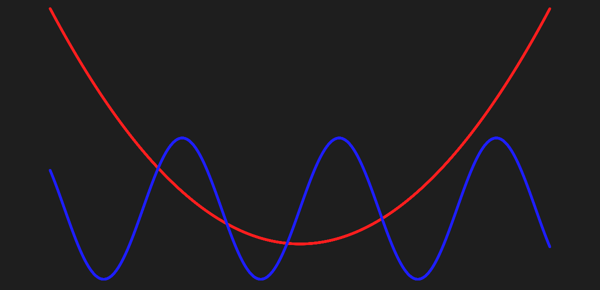
Two Functions

The (red) function below is: $y_{0} = x^2$

The (blue) function below is: $y_{1} = 30sin(x) + 15$

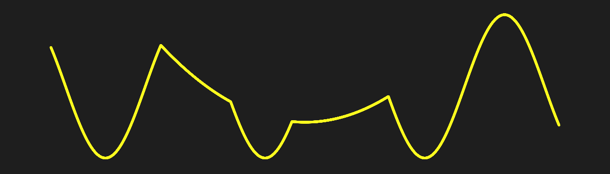
Min of the Two Functions

The (yellow) function below is: $y = min(y_{0}, y_{1})$

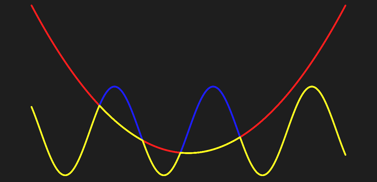
without the original functions:

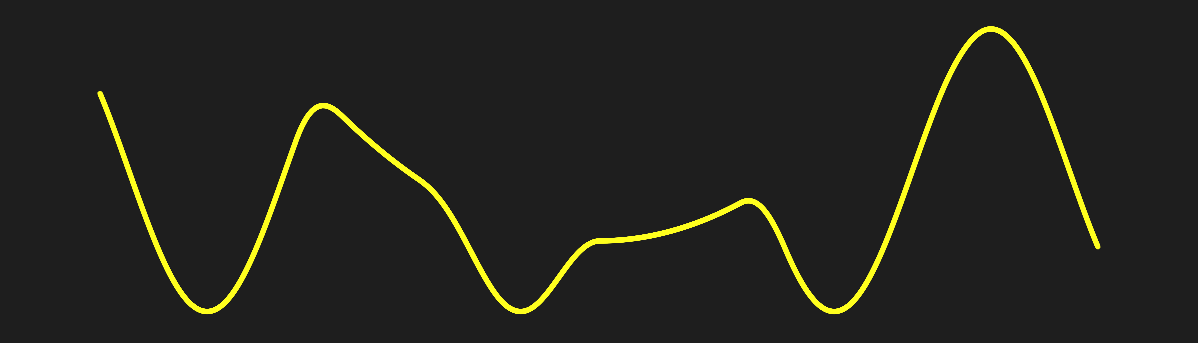
Smooth Min Function Applied

Now using the smooth min function instead of min: $y = SmoothMin(y_{0}, y_{1})$

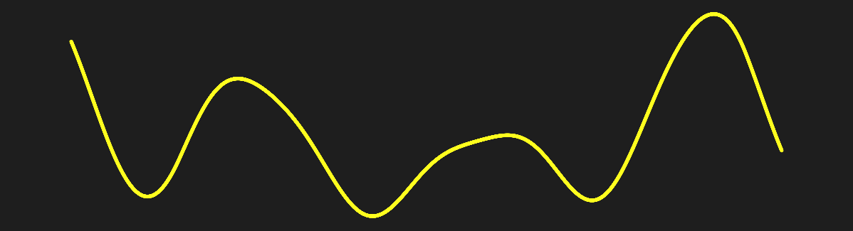
with more smoothing applied (a larger k value):

Smooth Min Code

  
function SmoothMin(a, b, k) {
	let h = Math.max(k-Math.abs(a-b), 0.0) / k;
	return Math.min(a, b) - h*h*k*(1.0 / 4.0);
}

Random Number with Bias

If a random number between $0$ and $1$ needs to be generated with a bias towards a certain number, the below function can be used⁴ ⁵. The function takes in a value $\left\{X \in \left[0,1 \right] \subset \mathbb{R}\right\}$, and a value $\left\{bias \in \left[0,1 \right) \subset \mathbb{R}\right\}$.

A $bias$ value of $0$ will mean no bias, while a $bias$ value closer to $1$ will mean lower values (closer to zero) are much more likely.

If a bias towards higher values (closer to one) is needed, then the output of the function can be subtracted from $1$:

$Output = 1 - BiasFunction(x, bias)$

  
function BiasFunction (x, bias) {
	let k = Math.pow(1-bias, 3);
	return (k*x) / (k*x - x +1);
}

The following graph shows the above function with $bias = 0$:

Now with a $bias = 0.6$:

Sources

Please see the sources below for more information regarding each topic:

Spherical Coordinate System - https://en.wikipedia.org/wiki/Spherical_coordinate_system ↩
Polar Coordinate System - https://en.wikipedia.org/wiki/Polar_coordinate_system ↩
Smooth Minimum Function - https://www.iquilezles.org/www/articles/smin/smin.htm ↩
Random Number with Bias 1 - https://www.youtube.com/watch?v=lctXaT9pxA0 ↩
Random Number with Bias 2 - https://www.shadertoy.com/view/Xd2yRd ↩

Interesting Algorithms